CINN Spline: Scalar & Representation Submodule
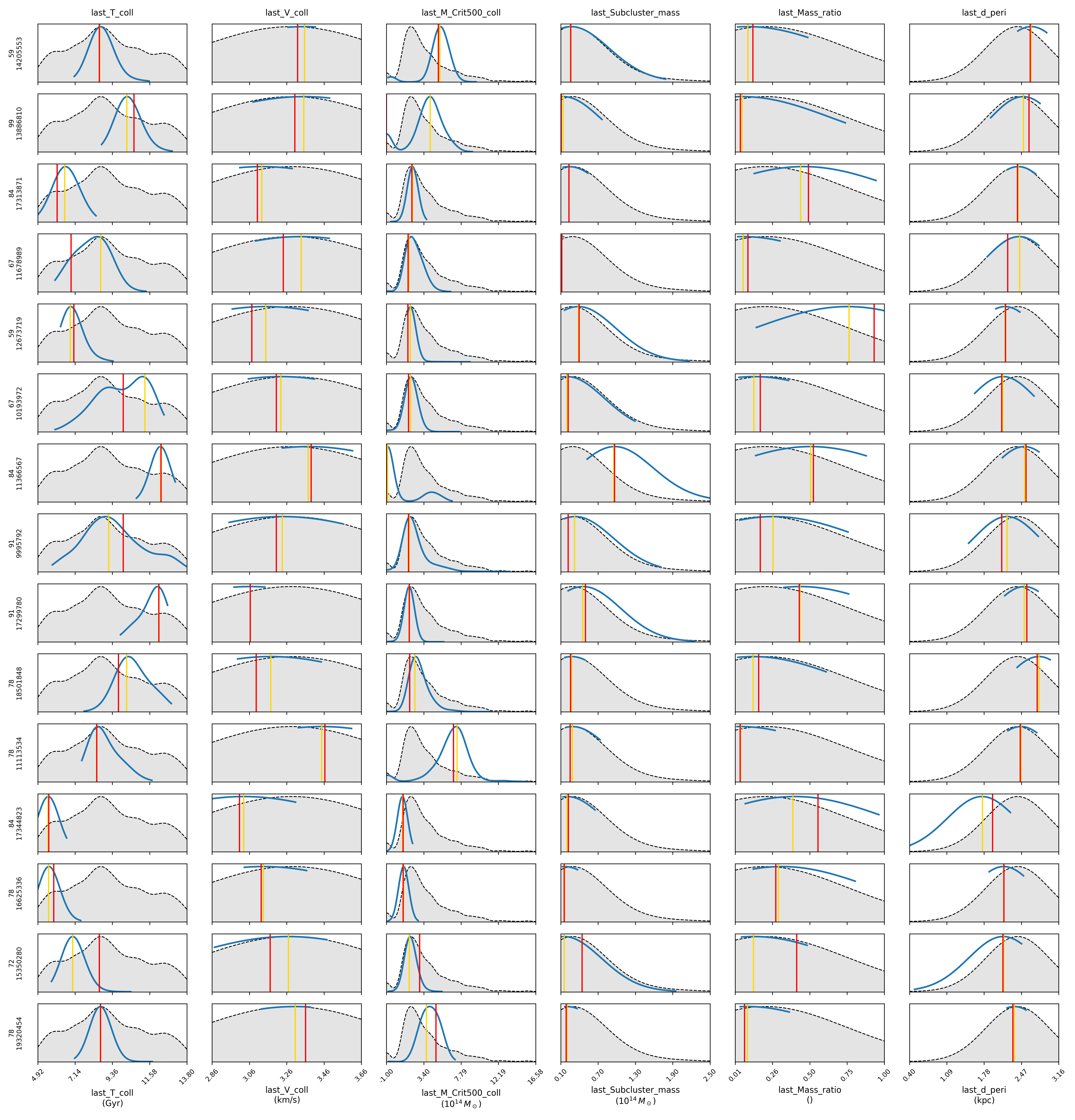
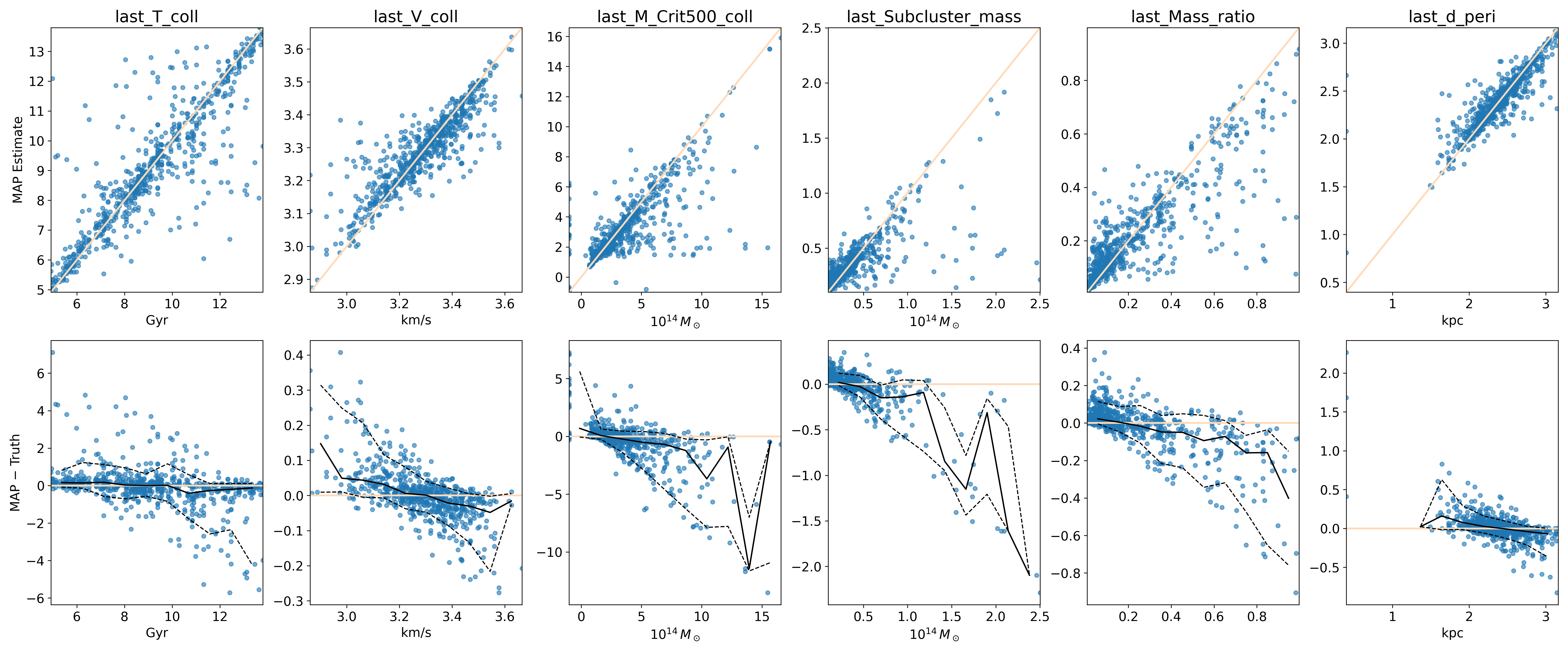
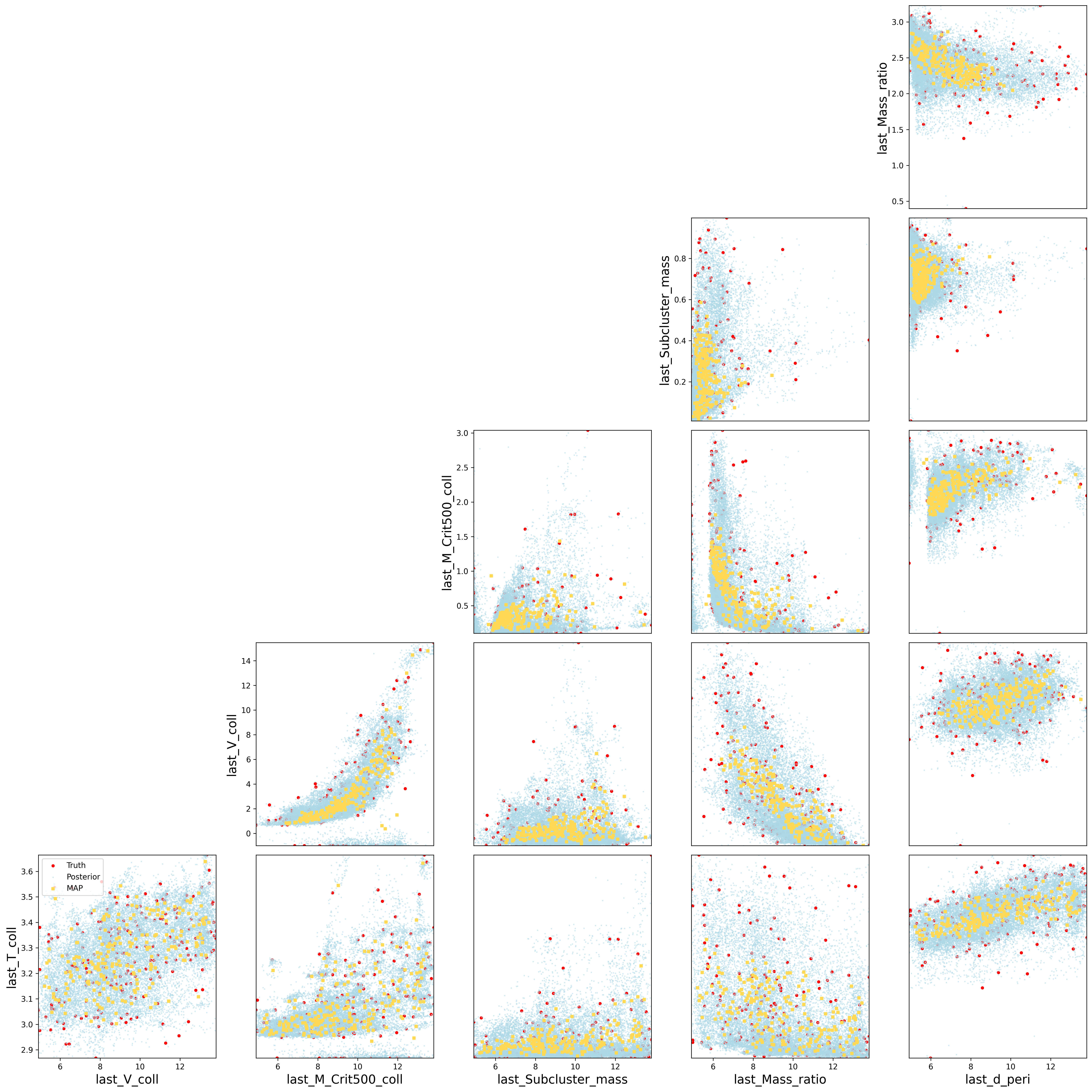
This project implements two complementary conditioning pipelines under the Conditional Invertible Neural Network (cINN) framework to infer galaxy cluster merger properties:
1. Scalar Pipeline
Inputs: Tabular observables (mass, radius, temperature, etc.), provided as CSV files.
Processing: Merge, clean, and scale features; split by unique
HaloID to prevent leakage; feed as conditioning vectors into the cINN.
2. Representation Pipeline
Inputs: Deep embeddings extracted from mock cluster images using
contrastive learning (SimCLR, NNCLR, DINO, etc.), stored in embeddings.npy.
Generated by our companion repo:
Shera1999/contrastive-learning
.
Processing: Optionally cluster embeddings via a Mixture‐of‐Experts,
then train one specialist cINN per cluster to better model heterogeneous regimes.
cINNs with Spline Coupling
At the core is a Conditional Invertible Neural Network built from alternating coupling blocks and permutations. Each block uses a rational-quadratic spline transform:
- VBLinear Bayesian layers capture weight uncertainty via the local reparameterization trick.
- A subnet predicts spline knots & slopes. Outside learned bounds, the transform is linear, guaranteeing invertibility and a tractable Jacobian.
-
Forward: data → latent
z, computinglog p(z) + log |det J|.
Reverse: samplez ~ 𝒩(0,I)to generate conditioned outputs.
Conditional INNs with Affine Coupling Blocks
In this variant, each coupling block splits its input into two halves: one
“frozen” and one “transformed.” A small subnet predicts scale (s)
and shift (t) factors from the frozen half and any conditioning
vector, then applies the affine transform:
- Forward: y₂′ = y₂ ⊙ exp(clamp · s) + t
- Inverse: y₂ = (y₂′ − t) ⊙ exp(−clamp · s)
- Log-determinant of Jacobian: log |det J| = Σ (clamp · s)
Random permutations between blocks ensure all dimensions interact, and the analytic Jacobian makes likelihood evaluation efficient.
Dual-Input Design
| Pipeline | Conditioning Vector x |
Folder |
|---|---|---|
| Scalar-only | 7 physical observables (CSV X.csv) |
scalar/ |
| Scalar + Embeddings |
Same observables + learned embeddings ( embeddings.npy) from
contrastive-learning
|
scalar+representation_space/ |
Feature Sensitivity Analysis
Alongside the flow models, an ensemble of MLPs is trained. By omitting each observable in turn, we measure the resulting Δ MAE (change in mean absolute error), revealing which features most influence each merger target.


